
Sturdy Statistics uses hierarchical, Bayesian priors to automatically separate the signal from the noise.
Our classification model has some unique features tailored to the real-world application of machine learning. It particularly stands out for its ability to a) train on small labeled datasets, and b) explain its predictions. Part of this performance comes from our use of Bayesian averaging, and part of it comes from our use of selective priors which identify and discard irrelevant information. By eliminating noise with its selective priors, our model makes more efficient use of labeled data, focusing information from the labels exclusively on the relevant portions of the data. These selective priors enable Sturdy Statistics models to deliver remarkably precise and efficient results.
This page demonstrates some of the features of our selective prior for regression. We will compare our favored regression model to L2 regression, sometimes called “ridge regression” in machine learning. Since we want to give L2 regression the best-possible chance of success in this comparison, we will hand-tune each L2 model like a professional data scientist would.1 At the same time, we will run the Sturdy Stats models just like a user of our API would, with no hand-tuning at all: the Sturdy Stats model is fully automatic and self-tuning. We hope to show just how effectively Sturdy Statistics can automate the task of a data scientist!
Example Problem: Recovering Regression Slopes
In order to have a simple, concrete demonstration, we’ll show results from a linear regression problem with an exact solution. We will generate the data according to a known formula and test how well each model recovers the data-generating formula. Since we know the true answer, we can easily assess how well each model performs.
We generate data of a given size according to: y = η · x + b + ε, where b = 0 is the intercept, and η = {5, 5, 5, 0, 0, 0, … , 0} is a vector of slopes, ε ∼ Normal(0, 1) is the observation noise, and x ∼ Normal(0, 1) are covariates sampled from a uniform standard normal distribution. Note that exactly three of the slopes are non-zero, with a value of 5, and all other slopes are exactly zero.
The python code to generate this data is as follows:
  from scipy import stats
  import numpy as np

  # number of "relevant" and "irrelevant" dimensions
  rel_dims, noise_dims = 3, 37

  N = 15                      # number of observations
  D = (noise_dims + rel_dims) # dimension of the data

  # true regression weights (which we will attempt to recover)
  η = np.hstack([
        np.ones(rel_dims) * 5.0,
        np.zeros(noise_dims) ])

  # covariates
  X = stats.norm(loc=0.0, scale=1.0).rvs(size=(N, D))

  # "true" dependent variable (noiseless)
  Y_ = np.einsum('nd,d->n', X, η)

  # "observed" dependent variable (with noise)
  ε = stats.norm(loc=0.0, scale=1.0).rvs(size=N)
  Y = Y_ + ε
Wide vs Tall Data:
When the number of data points N ≪ D
With N noiseless and uncorrelated data points, ordinary least squares can identify up to N-1 model parameters. If the covariates are correlated, or if the observations have noise, as all data do, this may reduce substantially. However, even if the data is perfect — uncorrelated and noise-free — it is often the case that the number of observations N is very much less than the dimensionality D of the problem. For example in genomics studies linking disease to genetic variations, you may have ∼105 gene traits (e.g., single nucleotide polymorphisms or SNPs) as covariates, but only ∼100 participants in the study. Alternatively, if you are classifying natural language, there are ∼170,000 words in the English language, many of which have multiple meanings. And there are a potentially infinite number of ideas for the words to be expressing. Yet you may need to train a classifier with fewer than 100 labeled examples. It is clear that you cannot solve such problems with a model which can identify only N-1 parameters!
This paradigm is known as wide data: in wide data problems, we have more complexity in the data than there is information about the data. In other words, the data alone does not and cannot fully specify the problem. This is to be contrasted with tall data, sometimes also called “big data.” In the tall data regime, the data has more information than complexity; in other words, the data repeats. Because of this, in tall data problems, you have essentially no uncertainty in the data. You can work with approximate models, and you can assume any errors caused by approximation will simply average out as you add more data. Thus, your approximations become better and better as you collect more and more data.
Much of machine learning presumes that you’re working with tall data. However, most real-world problems are wide: if you work in election forecasting or in targeted marketing, your data points are individual persons; since no two people are alike, you will never see repeats, and you and cannot simply beat down uncertainty with more data — more data would also bring more complexity! If you work with natural language data, you will find that no two documents, conversations, or manuscripts are exactly alike; there is again far more complexity in the data than there is information about it. Genome data is wide, as is virtually all data in the natural sciences. Wide data is an incredibly important regime, and it is not well addressed by “big data” techniques. The next section demonstrates that Sturdy Stats models are very well-adapted for wide data problems.
Regression on Wide Data Problems
We will illustrate the wide data regime with a simple example: we will do linear regression with Drel = 3 meaningful covariates and Dnoise = 37 coordinates, for a total dimensionality D = 40. The meaningful coordinates all have a linear coefficient ηrel = 5; the noise dimensions of course have a coefficient ηnoise = 0. From this, we will generate N = 15 observations with a noise scale ε = 1.0. Thus, we have a signal much greater than the noise (ηrel ≫ ε), along with enough data to measure the signal (N ≫ Drel). However, we do not have enough data to constrain all of the noise dimensions: N ≪ Dnoise. Moreover, the scale of the noise is similar to the scale of the covariates (x ≈ ε). Thus, a linear model could in principle fit the data, but only if it can identify and ignore the noise coordinates.
The following figure shows fits to this data using both standard L2 regression and the Sturdy Stats model:
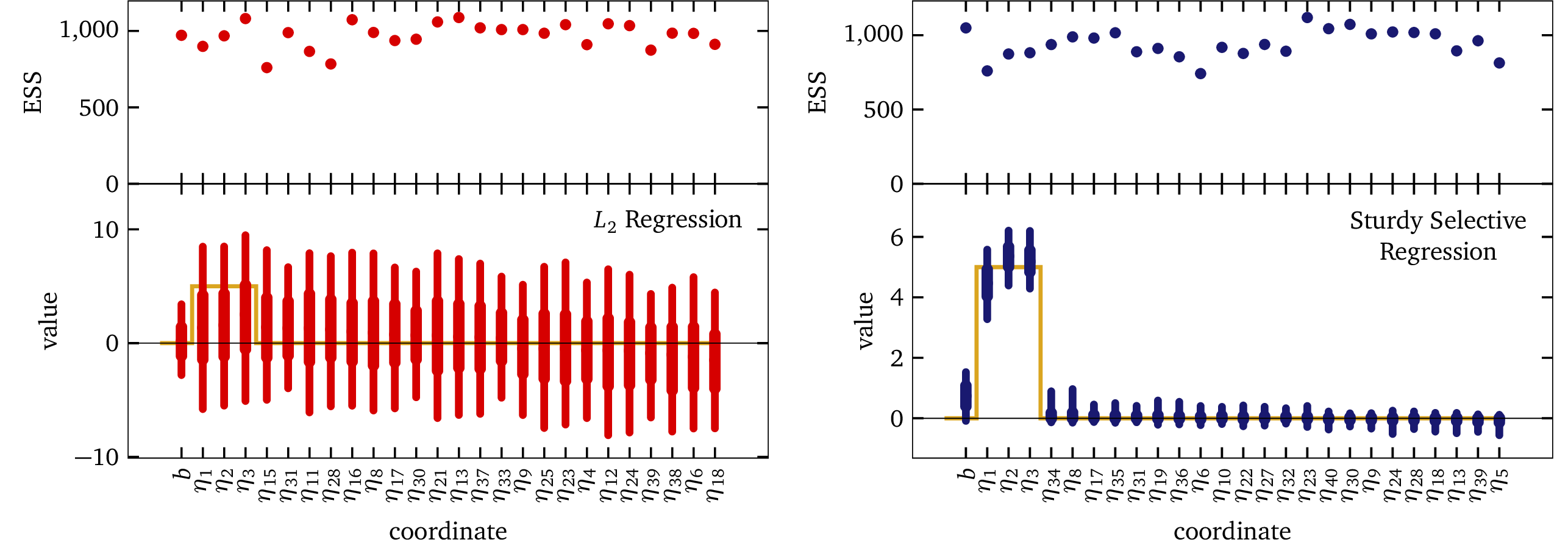
In each panel of the figure above, the gold curve shows the correct solution, with ηrel = 5; and ηnoise = 0, and with an intercept b = 0. The blue bars in the right-hand panel show that the Sturdy Stats selective regression has recovered this solution remarkably accurately: each and every one of our model’s estimates intersects the true solution. Recall that a Bayesian analysis does not simply produce a point estimate for each model parameter; instead, it produces a full probability distribution over that parameter’s value. The thick bar shows the 50% confidence interval (i.e., there is a 50% chance the value is inside the thick bar), and the thin bar shows the 90% confidence interval. Our model has cleanly separated the relevant dimensions from the noise dimensions, and is has used the data to make inference about the relevant dimensions; there is plenty of data for it to do so.
The red points in the left-hand panel of the plot show results for typical L2 regression. We can see that this model did not perform well at all; in fact, the bars are so large that it is almost hard to see the correct solution plotted underneath them. In this example, we cheated and “tuned” the L2 model for this problem: we programmed in that the intercept should have a scale ≲1, and that the coefficients should each have a scale ≲5. We have furthermore programmed in that the noise has a scale ≲1; in other words, most of the expected answer comes already baked into the model! The behavior you see here is considerably better than you would see “out of the box,” or in any realistic scenario. Despite such strong hints about the true solution, the L2 model inferred virtually nothing about the data; the model threw up its hands and estimated ±5 for every parameter in the problem. In other words, the model gave us no more information than we explicitly programmed into it. As expected based on counting parameters, ordinary linear regression is entirely unable to fit this dataset.
Both models do, however, show excellent computational performance. In this example, we ran our MCMC sampler for 1,000 steps. The top panel of each plot shows the effective sample size (ESS) for each parameter. In all cases, this number is close to 1,000. Our sampler performs extremely well, and extremely efficiently, for both models!
Full Distribution Functions Over Parameters
Because the above plot shows the L2 and Sturdy Stats models on different scales, it’s hard to see just how different the two are. In the following plot, we show the two models on the same axes. The left panel shows posterior distributions for the weight on a relevant dimension (which should be 5), while the right panel shows posterior distributions for the weight on an irrelevant dimension (which should be 0).

In the right-hand plot, the Sturdy Stats model produces a “spike” distribution right on the correct answer; the L2 model produced a “slab” distribution which is essentially uniform over the domain. The spike is so narrow, and the slab so broad, that they are both almost difficult to see! (In fact we had to multiply the slab by a factor of 4 to even render it visible.) Again, you can see that the L2 model simply gave up and output ± 5 for each parameter, simply regurgitating the information that was programmed into it. The Sturdy Stats model, on the other hand, confidently and precisely identified the correct solution.
We see similar behavior in the left-hand plot: while the L2 model simply regurgitates its prior, the Sturdy Stats model produces a sharp, informative distribution exactly centered on the correct solution.
Direct Visualization Against the Data
Thus far, we have inspected how well our model recovers the true data generating process in our test problem. Such investigation is essential for testing models and for establishing their trustworthiness. But it is also somewhat abstract; moreover, it is not possible in real-world problems, where the data generating process is unknown. So it is also helpful to check our model predictions against the actual data.
In the following plot, black points represent the data and the y axis shows the dependent, or target, variable. Each x axis shows its labeled covariate; each plot shows a single one of the data’s 40 dimensions. The top row of plots show the 3 relevant dimensions, which should have a slope of 5. This true slope is marked with a black line. The second row of plots shows 3 of the “noise” dimensions, which should have a slope of 0. This true slope is again marked with a black line.
As before, we show results for the L2 model in red, and for the Sturdy Stats model in blue. We represent the uncertainty with shaded regions; the darker region encloses 50% of the probability, and the lighter region encloses 90% of the probability.
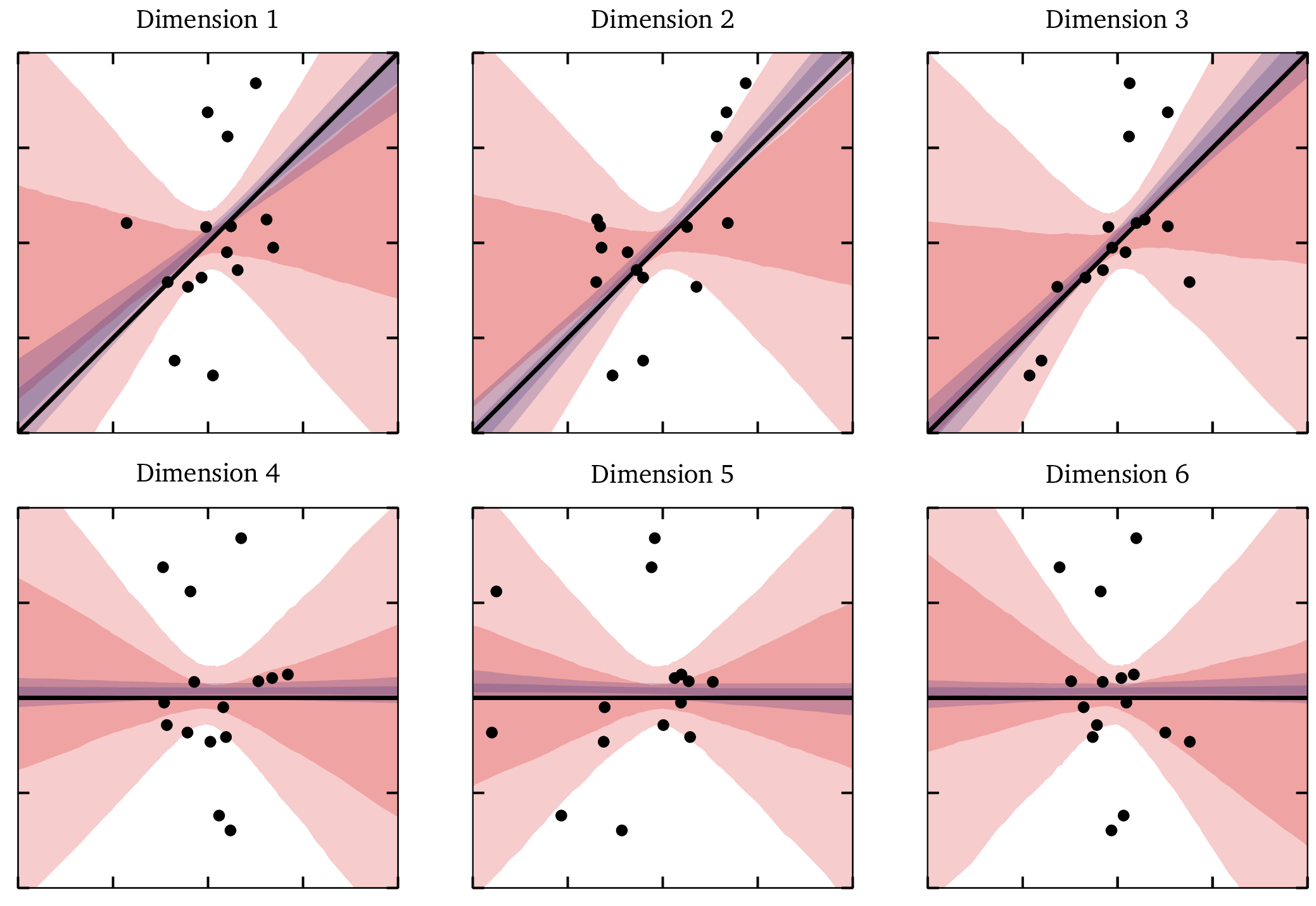
First and foremost, this plot shows just how little information there is in this data, and what a challenge it is to recover the slopes from it! I think you would be hard-pressed to discern the relevant from the irrelevant dimensions by visual inspection alone.
You can see that the Sturdy Stats model closely reproduces the true solution. You can also see that the L2 model struggles to extract information from the data: the uncertainty bands are so wide that the cover much of the parameter space. In each of the three relevant dimensions, the L2 model failed to identify even the sign of the slope within the 50% confidence region, much less its magnitude.
Tall Data: When the number of data points N ≳ D:
If we increase the data set size to 45, such that there are more data points than dimensions, the L2 model is able to function, and it does converge to the correct solution. However, it is important to note that even in this regime, L2 regression does not perform as well as the Sturdy Stats selective regression model. While L2 regression begins to narrow its confidence intervals and to lock onto the correct solution, its estimates remain less accurate, and far less precise than the results achieved by Sturdy Stats. Our model not only converges more quickly but also provides sharper, more informative intervals for parameter estimates, distinguishing relevant dimensions from noise with far greater clarity.
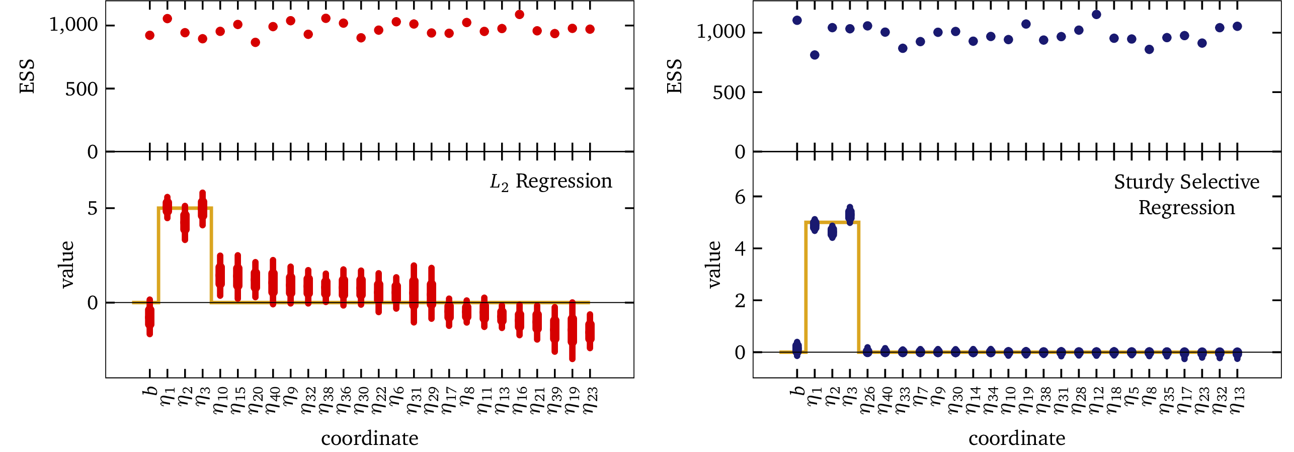
Moreover, relying on an increase in sample size to achieve comparable performance highlights a critical limitation of L2 regression: the requirement for N≥D to even function. This is an unrealistic expectation in many real-world scenarios, such as genomics (with millions of SNPs compared to limited samples) or natural language processing (where the number of topics or dimensions dwarfs the available training data). In contrast, the Sturdy Stats regression model thrives in both tall and wide data regimes, making it a practical and robust solution for modern high-dimensional data challenges.
Very Sparse Data:
When we reduce the dataset to just 10 points, it may initially seem as though the Sturdy Stats model begins to struggle. However, closer inspection reveals that this is not a failure at all. The quantile bars suggest broad uncertainty in the weights for the relevant dimensions, but a deeper examination of the full distribution tells a different story: the model produces a bimodal distribution which is not well represented by the quantile bars.
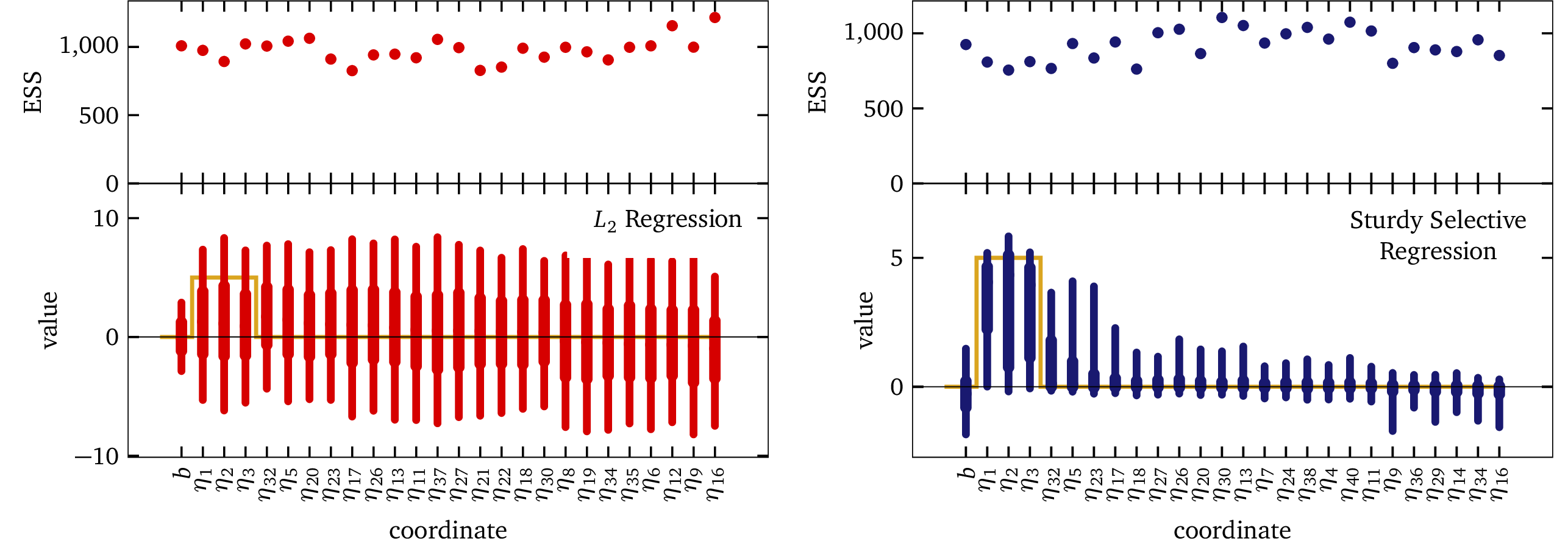 In this case, the model has identified a mixture of solutions — one centered at zero and another, much stronger mode at the correct value of 5.
This reflects the model’s nuanced understanding of the data.
Given the limited evidence, the model cannot conclusively determine that all three relevant dimensions matter.
Yet remarkably, it still accounts for the possibility that they do, and in that case, the solution is precisely correct.
In this case, the model has identified a mixture of solutions — one centered at zero and another, much stronger mode at the correct value of 5.
This reflects the model’s nuanced understanding of the data.
Given the limited evidence, the model cannot conclusively determine that all three relevant dimensions matter.
Yet remarkably, it still accounts for the possibility that they do, and in that case, the solution is precisely correct.

Effectively, the model is saying, “Given the lack of evidence, I can’t be certain these dimensions are all important. But if they are, their weight is 5.” At the same time, for the irrelevant dimensions, the model confidently assigns a weight of 0, demonstrating its ability to separate signal from noise even in extremely sparse data regimes. In stark contrast, the L2 regression model fails catastrophically, unable to extract meaningful information from the data and providing no useful insights.
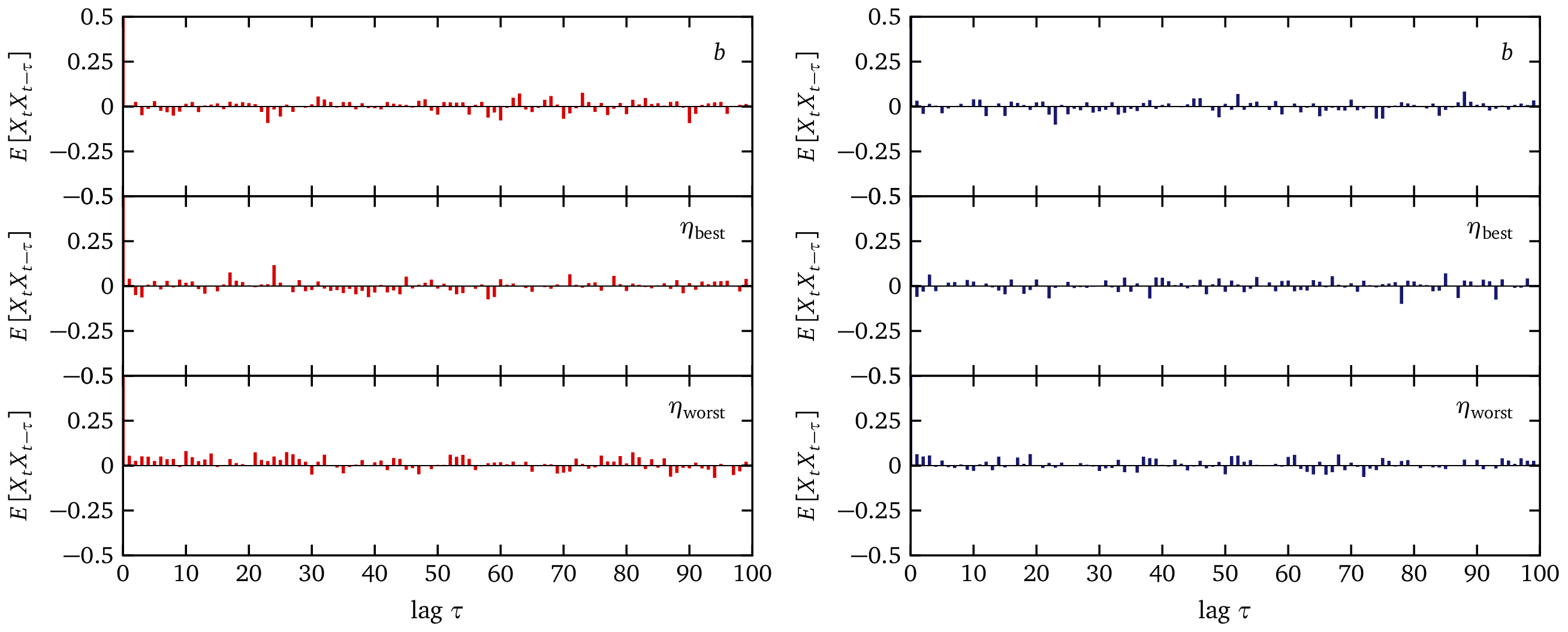
Convergence, Auto-Correlation, and Effective Sample Size
The figure below E[Xt Xt-τ]
Notes
1 In this case, that same data scientist also created the dataset, so he knows with certainty how to tune the model. This gives an absolutely unfair and unrealistic advantage to the L2 model! ↩