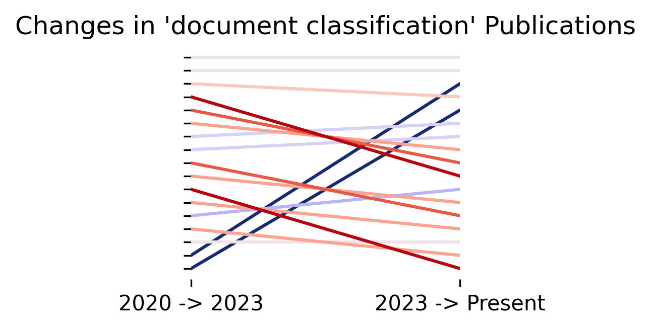
Changes in Novartis’ News Coverage
3 min
In the following notebook, we will be recreating Sturdy Statistics’ DeepDive page using the sturdy-stats-sdk.
In this notebook we will reproducing this deep dive analysis on all the hacker news comments that discuss duckdb (our favorite data processing engine at Sturdy Statistics).
pip install sturdy-stats-sdk pandas numpy plotly
from IPython.display import display, Markdown, Latex
import pandas as pd
import numpy as np
import plotly.express as px
from sturdystats import Index, Job

from pprint import pprint## Basic Utilities
px.defaults.template = "simple_white" # Change the template
px.defaults.color_discrete_sequence = px.colors.qualitative.Dark24 # Change color sequence
def procFig(fig, **kwargs):
fig.update_layout(plot_bgcolor= "rgba(0, 0, 0, 0)", paper_bgcolor= "rgba(0, 0, 0, 0)",
margin=dict(l=0,r=0,b=0,t=30,pad=0),
title_x=.5,
**kwargs
)
fig.layout.xaxis.fixedrange = True
fig.layout.yaxis.fixedrange = True
return fig
def displayText(df, highlight):
def processText(row):
t = "\n".join([ f'1. {r["short_title"]}: {int(r["prevalence"]*100)}%' for r in row["paragraph_topics"][:5] ])
x = row["text"]
res = []
for word in x.split(" "):
for term in highlight:
if term in word.lower() and "**" not in word:
word = "**"+word+"**"
res.append(word)
return f"<em>\n\n#### Result {row.name+1}/{df.index.max()+1}\n\n#### {row['published']}\n\n"+ t +"\n\n" + " ".join(res) + "</em>"
res = df.apply(processText, axis=1).tolist()
display(Markdown(f"\n\n...\n\n".join(res)))Sturdy Statistics integrates directly with Hacker News. Below we query the hackernews_comments integration for all comments that mention duckdb.
Training a model on our hacker news integration takes anywhere from 5-10 minutes. This step is optional and you can instead proceed with our public duckdb analysis index.
index = Index(id="index_1da1f1bf6b3d4347af5d22b38708357c")

# Uncomment the line below to create and train your own index
# index = Index(name="hackernews_duckdb")

if index.get_status()["state"] == "untrained":
    index.ingestIntegration("hackernews_comments", "duckdb", args=dict(num_intervals=9))
    job = index.train(dict(subdoc_hierarchy=False), fast=True, wait=False)
    print(job.get_status())
    # job.wait() # Sleeps until job finishes
Found an existing index with id="index_1da1f1bf6b3d4347af5d22b38708357c".In this section, we will demonstrate how to produce the two core visualization in their simplest form: the sunburst and the time trend plot.
index = Index(id="index_1da1f1bf6b3d4347af5d22b38708357c")Found an existing index with id="index_1da1f1bf6b3d4347af5d22b38708357c".Our bayesian probabilistic model learns a set of high level topics from your corpus. These topics are completely custom to your data, whether your dataset has hundreds of documents or billions. The model then maps this set of learned topics to single every word, sentence, paragraph, document, and group of documents to your dataset, providing a powerful semantic indexing.
This indexing enables us to store data in a granular, structured tabular format. This structured format enables rapid analysis to complex questions.
df = index.topicSearch()
df.head(5)[["short_title", "topic_group_short_title", "topic_id", "mentions", "prevalence"]]| short_title | topic_group_short_title | topic_id | mentions | prevalence | |
|---|---|---|---|---|---|
| 0 | DuckDB vs SQLite | DuckDB Specifics | 57 | 739.0 | 0.064246 |
| 1 | Data Lakehouse Integration | Data Integration | 64 | 653.0 | 0.054708 |
| 2 | Single Node vs. Distributed Systems | Data Processing and Querying | 23 | 624.0 | 0.054172 |
| 3 | DuckDB Discussions | DuckDB Specifics | 59 | 662.0 | 0.051199 |
| 4 | Building Together | User Engagement | 25 | 523.0 | 0.045821 |
We can see there are two names: short_title and topic_group_short_title. The topic group is a high level thematic category while a topic is a much more granlular annotation.
A dataset can have hundreds of topics, but ussually only 20-50 topic groups. This hierarchy is extremly useful for organizing and exploring data in hierarchical formats such as sunbursts.
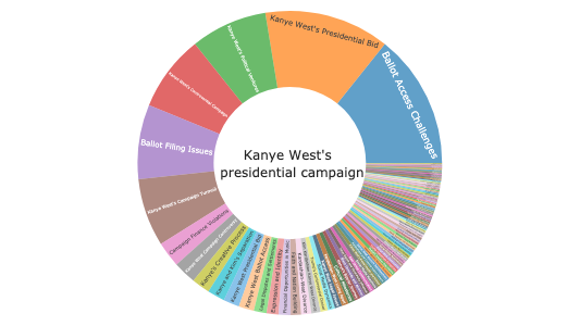
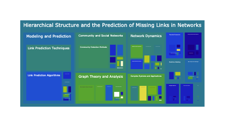
The Inner circle of the sunburst is the title of the plot. The middle layer is the topic groups. And the leaf nodes are the topics that belong to the corresponding topic group. The size of each node is porportional to how often it shows up in the dataset.
df["title"] = "DuckDB Hacker <br> News Comments"
fig = px.sunburst(
    df,
    path=["title", "topic_group_short_title", "short_title"],
    values="prevalence", hover_data={"topic_id": True}
)
procFig(fig, height=500).show()SEARCH_QUERY = "pandas"When you submit a search query, our indexing model maps your query to its thematic contents. Our index is a unified Bayesian probabilistic model and we use a statistically meaningful scoring metric called hellinger distance to score each candidate excerpt within your Index. Unlike cosine distance whose values are not well defined and can be used only to rank, the hellinger distance score defines the percentage of a document that ties directly to your theme.
This well defined score enables not only search ranking, but semantic search filter as well with the ability to define a hand-selected hard cutoff.
docdf = index.query(SEARCH_QUERY, semantic_search_cutoff=.2, limit=100)
displayText(docdf.sample(2), highlight=[SEARCH_QUERY])
“Strongest support” is probably Pandas, in that it is very widely used and easy to get help with. DuckDB lets you write SQL and is very fast.
…
Lancedb/lance works with **[Pandas,** DuckDB, Polars, Pyarrow,];https://github.com/lancedb/lance
You will notice that accompanying each excerpt is a set of tags. These tags are the exacts some topics that we visualized in the sunburst. The topicSearch (and all other topic apis) are simple rollups over segments of data you defined.
The Sturdy Statistics API offers a unified interface for query thematic content as well. This leverages our vertically integrated thematic search. The search query you provide here matches on the exact same set of documents as the query above, but instead of providing the data, it provides a rollup on the thematic content of the data.
topic_df = index.topicSearch(SEARCH_QUERY)
topic_df["title"] = f"DuckDB <br> Comments::{SEARCH_QUERY}"
fig = px.sunburst(topic_df, path=["title",  "topic_group_short_title", "short_title"], values="prevalence", hover_data={"topic_id": True})
procFig(fig, height=500).show()We can select any point above and pull out the actual excerpts that comprise it. Let’s say we are interested diving into the topic Complex SQL Queries (topic 62). We can easily query our index to pull out the matching excerpts.
This query is filtering on documents that match on pandas as well as the topic Complex SQL Queries.
topic_id = 62
row = topic_df.loc[topic_df.topic_id==topic_id]
row| short_title | topic_id | mentions | prevalence | one_sentence_summary | executive_paragraph_summary | topic_group_id | topic_group_short_title | conc | entropy | title | |
|---|---|---|---|---|---|---|---|---|---|---|---|
| 7 | Complex SQL Queries | 62 | 89.0 | 0.036064 | The theme revolves around the challenges and s... | The discussion highlights the difficulties SQL... | 11 | Data Processing and Querying | 26.748852 | 6.478961 | DuckDB <br> Comments::pandas |
docdf = index.query(SEARCH_QUERY, topic_id=topic_id, semantic_search_cutoff=.2, limit=100)
print("Search:", SEARCH_QUERY, "Topic:", row.short_title.iloc[0])
displayText(docdf.iloc[[0, -1]], highlight=["duckdb", SEARCH_QUERY, "faster", "complex", "sql", "aggregate", "relational", "api"])
Search: pandas Topic: Complex SQL Queries
I’ve been using duckdb instead of Pandas these days because it’s much faster on larger datasets plus I can write more compact and complex SQL than I can Pandas constructs. The fact that duckdb can query in memory Pandas dataframes faster than Pandas itself is a plus.
…
A missed opportunity here is the redundant [AGGREGATE** sum(x) GROUP BY y]. Unless you need to specify rollups, [AGGREGATE** y, sum(x)] is a sufficient syntax for group bys and duckdb folks got it right in the relational api.
Sturdy Statistics embeds all of its semantic information into a tabular format. It directly exposes this tabular format through the queryMeta api.
In fact, all of our topic apis directly query the same tabular data structures that we expose in the queryMeta api.
Similar to our topic api, Sturdy Statistics integrates its semantic search directly into its sql api, enabling powerful sql analyses. For this analysis we will also change up our search query to explore new content.
df = index.queryMeta("""
SELECT
    date_trunc('month', published::DATE) as month,
    count(*) as comments
FROM doc
GROUP BY month
ORDER BY month
""",
SEARCH_QUERY)

fig = px.line(df,
"month", "comments",
line_shape="hvh",
title=f"DuckDB Comments::{SEARCH_QUERY} over Time"
)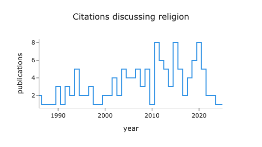
procFig(fig)Just as we were able to focus in on a specifc topic in our query, we can also query topics directly within sql.
Below, we query the number of paragraphs that mention the topic Complex SQL Queries (topic 62).
topic_id = 62
df = index.queryMeta(f"""
SELECT
    date_trunc('month', published::DATE) as month,
    sum((sparse_list_extract(
        {topic_id+1}, -- 1 indexed
        c_mean_avg_inds,
        c_mean_avg_vals
    ) > 2.0)::INT) as comments
FROM paragraph
GROUP BY month
ORDER BY month
""",
search_query=SEARCH_QUERY, semantic_search_cutoff=.2)
fig = px.line(df, "month", "comments", line_shape="hvh", title=f"DuckDB Comments::{SEARCH_QUERY}")
procFig(fig).show()assert df.comments.sum() == len(docdf)Every high level visualization or rollup can be instantly tied back to the original data, no matter how granular or complex.
Let’s saw we want to pull out all hacker news comments that discuss pandas and mention the topic Complex SQL Queries that happened in 2025. That is a simple API call
docdf = index.query(SEARCH_QUERY, topic_id=topic_id, semantic_search_cutoff=.2, limit=100, filters="published > '2025-01-01'")
print("Search:", SEARCH_QUERY, "Topic:", row.short_title.iloc[0])
displayText(docdf.iloc[[0, -1]], highlight=["duckdb", SEARCH_QUERY, "faster", "complex", "sql", "aggregate", "relational", "api"])
Search: pandas Topic: Complex SQL Queries
I write a lot of SQL anyway, so this approach is nice in that I find I almost never need to look up function syntax like I would with Pandas, since it is just using DuckDB SQL under the hood, but removing the need to write select * from ... repeatedly. And when you’re ready to exit the data exploration phase, its easy to gradually translate things back to “real **SQL”.
**
…
Similar functionality already exists in some SQL implementations, notably **DuckDB:
**
assert df.loc[df["month"] >= "2025-01-01"].comments.sum() == len(docdf)While it is possible to reconstruct our apis from scratch, the topicSearch is extremely helpful for simple multi-topic analysis. Below we are going to query the topical content of every quarter combination that discusses pandas with a simple for loop.
dfs = []
## Get the quarter in which the search query shows up
data = index.queryMeta(
"SELECT distinct date_trunc('quarter', published::DATE) as quarter from paragraph",
search_query=SEARCH_QUERY, semantic_search_cutoff=.2
)
## For each quarter, get a rollup of topics
for quarter in data.quarter.tolist():
tmp = index.topicSearch(query=SEARCH_QUERY, filters=f" date_trunc('quarter', published::DATE)='{quarter}'", semantic_search_cutoff=.2).head(30)
tmp["quarter"] = quarter
dfs.append(tmp)
df = pd.concat(dfs, ignore_index=True)
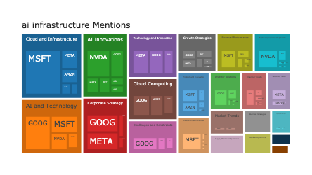
df["title"] = SEARCH_QUERY + " Mentions"
## Filter by the ones that show up a lot
top_topics = df.loc[df.mentions >10].topic_id.unique()
df = df.loc[df.topic_id.apply(lambda x: x in top_topics)]
df.sample(5)| short_title | topic_id | mentions | prevalence | one_sentence_summary | executive_paragraph_summary | topic_group_id | topic_group_short_title | conc | entropy | quarter | title | |
|---|---|---|---|---|---|---|---|---|---|---|---|---|
| 513 | Data Lakehouse Integration | 64 | 13.0 | 0.059765 | This theme explores the integration and utiliz... | The documents highlight the emergence of data ... | 14 | Data Integration | 14.232922 | 5.675903 | 2023-01-01 | pandas Mentions |
| 585 | Complex SQL Queries | 62 | 3.0 | 0.018038 | The theme revolves around the challenges and s... | The discussion highlights the difficulties SQL... | 11 | Data Processing and Querying | 26.748852 | 6.478961 | 2022-04-01 | pandas Mentions |
| 515 | DuckDB vs SQLite | 57 | 12.0 | 0.037353 | DuckDB, an OLAP columnar database, is optimize... | The discussions surrounding DuckDB emphasize i... | 4 | DuckDB Specifics | 16.041576 | 5.773169 | 2023-01-01 | pandas Mentions |
| 542 | Complex SQL Queries | 62 | 2.0 | 0.099413 | The theme revolves around the challenges and s... | The discussion highlights the difficulties SQL... | 11 | Data Processing and Querying | 26.748852 | 6.478961 | 2021-04-01 | pandas Mentions |
| 303 | Complex SQL Queries | 62 | 1.0 | 0.108685 | The theme revolves around the challenges and s... | The discussion highlights the difficulties SQL... | 11 | Data Processing and Querying | 26.748852 | 6.478961 | 2020-10-01 | pandas Mentions |
fig = px.area(
    df.sort_values(["mentions"], ascending=False),
    x="quarter",
    y="mentions",
    color="short_title",
    title=f"DuckDB vs {SEARCH_QUERY} Discussion",
    line_shape="hvh"
)
fig = procFig(fig)
figfrom sturdystats import Index
index = Index("Custom Analysis")
index.upload(df.to_dict("records"))
index.commit()
index.train()
# Ready to Explore
index.topicSearch()