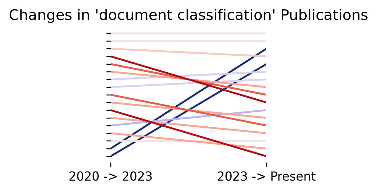
Changes in Novartis’ News Coverage
3 min
pip install sturdy-stats-sdk pandas numpy plotly
from IPython.display import display, Markdown, Latex
import pandas as pd
import numpy as np
import plotly.express as px
from sturdystats import Index, Job

from pprint import pprint## Basic Utilities
px.defaults.template = "simple_white" # Change the template
px.defaults.color_discrete_sequence = px.colors.qualitative.Dark24 # Change color sequence
def procFig(fig, **kwargs):
fig.update_layout(plot_bgcolor= "rgba(0, 0, 0, 0)", paper_bgcolor= "rgba(0, 0, 0, 0)",
margin=dict(l=0,r=0,b=0,t=30,pad=0),
**kwargs
)
fig.layout.xaxis.fixedrange = True
fig.layout.yaxis.fixedrange = True
return fig
def displayText(df, highlight):
def processText(row):
t = "\n".join([ f'1. {r["short_title"]}: {int(r["prevalence"]*100)}%' for r in row["paragraph_topics"][:5] ])
x = row["text"]
res = []
for word in x.split(" "):
for term in highlight:
if term in word.lower() and "**" not in word:
word = "**"+word+"**"
res.append(word)
return f"<em>\n\n#### Result {row.name+1}/{df.index.max()+1}\n\n##### {row['ticker']} {row['pub_quarter']}\n\n"+ t +"\n\n" + " ".join(res) + "</em>"
res = df.apply(processText, axis=1).tolist()
display(Markdown(f"\n\n...\n\n".join(res)))index = Index(id="index_4fd50a6fa7444cbcb672db636d811f4b")
# Uncomment the line below to create and train your own index
# index = Index(name="Radford_Neal_Publications")
if index.get_status()["state"] == "untrained":
# https://www.semanticscholar.org/author/Radford-M.-Neal/1764325
author_id = "1764325"
index.ingestIntegration("author_cn", author_id)
index.train(dict(burn_in=1200, subdoc_hierarchy=False), fast=True)
print(job.get_status())
# job.wait() # Sleeps until job finishesFound an existing index with id="index_4fd50a6fa7444cbcb672db636d811f4b".Our bayesian probabilistic model learns a set of high level topics from your corpus. These topics are completely custom to your data, whether your dataset has hundreds of documents or billions. The model then maps this set of learned topics to single every word, sentence, paragraph, document, and group of documents to your dataset, providing a powerful semantic indexing.
This indexing enables us to store data in a granular, structured tabular format. This structured format enables rapid analysis to complex questions.
index = Index(id="index_4fd50a6fa7444cbcb672db636d811f4b")
df = index.topicSearch()
df.head()
Found an existing index with id="index_4fd50a6fa7444cbcb672db636d811f4b".| short_title | topic_id | mentions | prevalence | one_sentence_summary | executive_paragraph_summary | topic_group_id | topic_group_short_title | conc | entropy | |
|---|---|---|---|---|---|---|---|---|---|---|
| 0 | Bayesian Machine Learning Models | 82 | 26.0 | 0.104794 | The theme encompasses various methodologies in... | This theme explores the application of Bayesia... | 2 | Machine Learning | 26.669127 | 7.259441 |
| 1 | Gaussian Process Regression | 26 | 19.0 | 0.095460 | The theme explores the flexibility and applica... | Gaussian Process (GP) regression models are a ... | 1 | Statistical Methods | 35.986237 | 7.213645 |
| 2 | Adaptive Slice Sampling | 83 | 14.0 | 0.071136 | The documents discuss methods for adaptive sli... | The theme revolves around adaptive slice sampl... | 0 | Sampling Techniques | 130.408447 | 6.885675 |
| 3 | Exact Summation Methods | 59 | 11.0 | 0.069014 | The discussed methods focus on achieving high ... | The provided examples illustrate advanced meth... | 1 | Statistical Methods | 17.029112 | 7.432269 |
| 4 | Asymptotic Variance in MCMC | 80 | 8.0 | 0.066469 | This theme explores methods to reduce asymptot... | The examined theme highlights various techniqu... | 1 | Statistical Methods | 20.888794 | 7.365510 |
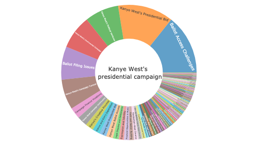
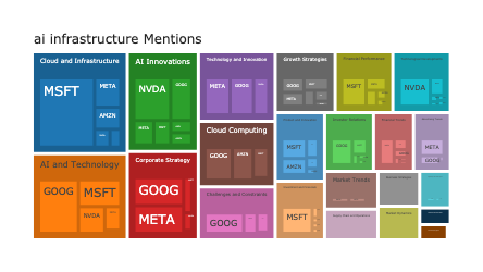
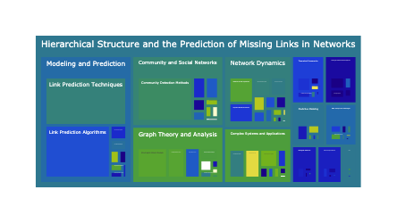
The following treemap visualizes the topics hierarchically: grouping the topics by the high level topic group. The size of each topic is porportional to the percentage of the time that topics shows up in Radford Neal’s publications.
fig = px.treemap(df, path=["topic_group_short_title", "short_title"], values="prevalence", hover_data=["topic_id"])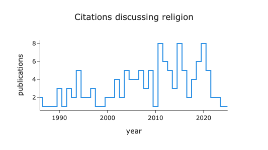
procFig(fig, height=500).show()Let’s say we are interested in learning more about the years during which Radford Neal published papers on Adaptive Slice Samling. The topic information has been converted into a tabular format that we can directly query via sql. We expose the tables via the queryMeta api. If we choose to, we can do all of our semantic analysis directly in sql.
row = df.loc[df.short_title == "Adaptive Slice Sampling"]
row| short_title | topic_id | mentions | prevalence | one_sentence_summary | executive_paragraph_summary | topic_group_id | topic_group_short_title | conc | entropy | |
|---|---|---|---|---|---|---|---|---|---|---|
| 2 | Adaptive Slice Sampling | 83 | 14.0 | 0.071136 | The documents discuss methods for adaptive sli... | The theme revolves around adaptive slice sampl... | 0 | Sampling Techniques | 130.408447 | 6.885675 |
row = row.iloc[0]

df = index.queryMeta(f"""
SELECT
    year(published::DATE) as year,
    count(*) as publications
FROM doc
WHERE sparse_list_extract({row.topic_id+1}, sum_topic_counts_inds, sum_topic_counts_vals) > 2.0
GROUP BY year
ORDER BY year
""")
fig = px.bar(df, x="year", y="publications", title=f"'{row.short_title}' Publications over Time",)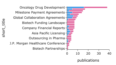
procFig(fig, title_x=.5)While it is possible to reconstruct our apis from scratch, the topicSearch is extremely helpful for simple multi-topic analysis. Just as you can do semantic analysis with SQL, you can also pass SQL to our topic apis.
Below we are going to query the topical content of every ticker, quarter combination that discusses AI Infrastructure with a simple for loop. Below pull out Radford Neals research focuses over each five year period of his career.
SEARCH_QUERY=""
dfs = []
for year in index.queryMeta("SELECT distinct ( (year(published::DATE)//5)*5 ) as year  FROM doc").year.dropna():
    tmp = index.topicSearch(SEARCH_QUERY, f"(year(published::DATE)::INT//5)*5 = {int(year)}").head(30)
    tmp["year"] = int(year)
    dfs.append(tmp)

df = pd.concat(dfs).rename(columns=dict(mentions="publications"))
df.sample(5)[["short_title", "topic_id", "publications", "year"]]| short_title | topic_id | publications | year | |
|---|---|---|---|---|
| 26 | Factorial Design Theory | 84 | 0.0 | 2005 |
| 11 | Mixture Model Techniques | 76 | 1.0 | 1995 |
| 2 | Adaptive Slice Sampling | 83 | 3.0 | 2000 |
| 20 | Anthropic Reasoning Challenges | 61 | 0.0 | 1990 |
| 1 | Embedded HMM Methods | 63 | 1.0 | 2015 |
Below visualze all of Radford Neal’s research topics broken down by time.
import duckdb
fig = px.bar(
    duckdb.sql("SELECT * FROM df ORDER BY year asc, publications desc").to_df(),
    x="year",
    y="publications",
    color="short_title",
    title=f"Radford Neal Publications over Time",
)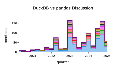
procFig(fig, title_x=.5, height=500)We can visualize the raw counts (mentions) or we can also visualize the prevalence field, which is the percentage of the total corpus that each topic makes up. Because we passed in a filter our topic search query, this prevalence is normalized by 5 year intervals
import duckdb
fig = px.bar(
    duckdb.sql("SELECT * FROM df ORDER BY year asc, prevalence desc").to_df(),
    x="year",
    y="prevalence",
    color="short_title",
    title=f"Radford Neal Publications over Time",
)
procFig(fig, title_x=.5, height=500)from sturdystats import Index
index = Index("Custom Analysis")
index.upload(df.to_dict("records"))
index.commit()
index.train()
# Ready to Explore
index.topicSearch()